Article Text

Abstract
Background Tobacco tax policy in Bosnia and Herzegovina (B&H) assumes a gradual annual increase in specific excise taxes on cigarettes. However, it is insufficient to reduce significantly consumption. This paper examines effects of the increase in cigarette prices and disposable income on cigarette demand in B&H by different income consumer groups.
Methods Based on the Household Budget Surveys and microdata from 2007, 2011 and 2015, we employed logit model to estimate prevalence and Deaton’s model to estimate intensity elasticity of cigarette demand for the sample of 21 424 households (9953 are smoking households) by different income groups. We used obtained elasticities and estimated the impact of tax increase on cigarette consumption and government revenue in three tax increase scenarios.
Results Ten per cent price increase would reduce the consumption of low-income households by 14%, as opposed to 9.9% for middle-income and 7% for high-income households. Low-income households would significantly increase the demand for cigarettes compared with high-income households if income increased. Increase in the specific excise tax by 25% would reduce cigarette consumption and increase government revenue, while the low-income group would experience a reduction in tax burden.
Conclusions Changes in prices have different impacts on tobacco prevalence and consumption of low-income compared with middle-income and high-income socioeconomic groups. Low-income households are most responsive to changes in prices and income. Thus, the poor in B&H would benefit from an increase in tobacco excise taxes and price.
- low/middle income country
- price
- taxation
- socioeconomic status
Data availability statement
Data are available on reasonable request. Data are available on reasonable request from the Agency of Statistics of Bosnia and Herzegovina.
Statistics from Altmetric.com
Introduction
Smoking prevalence and smoking intensity in Bosnia and Herzegovina (B&H) are extremely high. Around 41.1% of adults in 2019 used various tobacco products, while most of them (40.0%) were daily smokers of ‘classic’ tobacco, with the majority smoking more than 20 cigarettes per day.1 Increase in tobacco taxes is one of the most efficient instruments for reducing the smoking prevalence and smoking intensity.2–4 Since 2009, tobacco tax policy in Bosnia and Herzegovina (B&H) consists of ad valorem (currently set at 42% of retail price) and a specific excise (currently set at 0.84 EUR per pack of 20 cigarettes). The policy assumes a gradual annual increase in the specific excise tax on cigarettes (0.077 EUR per year per pack). However, these gradual increases have been insufficient to significantly reduce consumption. Additionally, as of 2020, policymakers in B&H have decided to freeze the increase in specific excise taxes proposed by the excise calendar.5 6 Previous research that was based on the data from Household Budget Survey (HBS) and conducted in B&H in 2011 and 2015, and the Deaton demand model,7 showed that if cigarette prices in B&H increased by 10%, the demand for cigarettes would decrease by 13.66%.8 Since the main driver of the increase in cigarette prices in B&H over the last decade has been the increase in excise taxes, the high response rate of cigarette demand to price increase indicates that increase in excise taxes is an effective tobacco control policy. However, defining the most appropriate tobacco tax and other polices requires an analysis of the effects of this policy on the smoking prevalence, smoking consumption of different socioeconomic groups, as well as on public revenue.
A limited number of studies were conducted in different low-income and middle-income countries (LMICs), such as B&H, to examine the impact of tobacco prices and income increase on demand for cigarettes in different socioeconomic groups. The study that analyses the price elasticity by income groups in Argentina9 shows that price increase by 10% reduces the cigarette consumption by 2.8% and that wealthier individuals are more price sensitive, in absolute value, than the poorer ones with respect to consumption but they are less price sensitive with respect to prevalence. The studies from Thailand and Moldova also show that the cigarette consumption in low-income socioeconomic groups is more responsive to changes in the price than those in high-income socioeconomic groups,10 11 while the study from Pakistan reveals that only smokers belonging to the low-income group are price sensitive.12
This paper examines price and income elasticity of the cigarette demand by three income groups in B&H. Reducing the demand for cigarettes can be reached by decreasing the prevalence of smoking or smoking intensity. Thus, we use a two-part model that is based on logistic regression to estimate prevalence elasticity and the Deaton demand method to estimate the elasticity intensity. The paper answers the question of which income group is most sensitive to price and income and provides a simulation effect of the specific tax increase on cigarette consumption and public revenue.
Data and methods
This analysis uses micro-level data, obtained from HBS13 in B&H in 2007, 2011 and 2015. The sample contains 21 424 households, of which 9953 are smoking households. Clusters are defined as a municipality x in the year and, according to this definition, 404 clusters are generated. In each cluster, on average, there are about 53 households. According to the criteria for applying the Deaton model, the households whose total expenditure is 5 SDs higher than the mean expenditure in the overall sample and the clusters with only one household are eliminated. So, the final number of observations for the calculation of the intensity elasticity is 9908 smoking households that belong to 389 clusters. Based on the distribution of household expenditures, the total sample of households is divided into three income groups: low, middle and high.
Two-part model
Many outcomes (yi), including smoking or tobacco use, have two fundamental statistical characteristics:
yi ≥ 0 for i=1… n1
yj = 0 for j = n1+1…n2
Cumulative distribution of cigarette consumption can be characterised as a mixed distribution that is part discrete and part continuous. If zero outcomes are large enough, as it is the case if we analyse which households among all do not smoke cigarettes, they cannot be ignored in the empirical modelling of these outcomes.
As the price of cigarettes increases, the household first decides whether to smoke or not. If the household decides to smoke, then they decide how many cigarettes they want to smoke. According to this decision-making process, the two-part model first estimates the probability of consumption or the prevalence elasticity (first part), and then estimates the quantity of consumption for positive outcomes conditional on positive purchases or the intensity elasticity (second part). The prevalence elasticity model uses a full sample of households, smoking and non-smoking, and estimates the probability of observing the positive versus zero consumption. The intensity elasticity model estimates the level of consumption conditional on positive outcomes (yi ≥ 0). Therefore, it uses only a subsample of smoking households and estimates the model of quantity of consumption for the positive outcomes conditional on positive purchase. This model can be estimated employing any econometric model for continuous variables, for example, ordinary least squares (OLS), generalised linear models (GLM) etc.
By employing the two-part model, the total expected smoking, say (yǀx), is calculated by using the advantage of the basic rule of probability:
(y ǀ x)=Pr (y>0) × (y ǀ>0)
that is, the total expected smoking is equal to the probability of smoking multiplied by the expected quantity of smoking for those who smoke. The two-part model allows for independence between the decision to smoke (first part of (yǀx) equation) and the decision how much to smoke (second part of (yǀx) equation). In the following part, we briefly describe the theoretical background of the models used to estimate the prevalence and intensity elasticity.
Prevalence elasticity model
The first part of the two-part model estimates the probability of smoking (Pr (yi > 0ǀx)) and analyses whether the cigarette prices impact the decision of a household to smoke, conditional on the set of independent variables. This estimation is governed by a parametric binary probability model – logit model, which models the probability of a positive outcome given a set of regressors (x):
Y=Pr (yi >0)=f(β1pi + β2ii+G X)
where yi is the cigarette consumption of the household i. Y is dependent variable, which takes value 1 for smoking households (if yi >0) and 0 for non-smoking households (yi=0); pi and ii are covariates of interest, price and income. X represents the vector of other covariates used in the analysis. The maximum likelihood procedure is used to fit the coefficients to the logit model.
Estimated coefficient of the defined logit model has no clear interpretation and does not represent marginal effects. To estimate prevalence elasticity, we calculate marginal effect of a covariate pi on Pr (y>0):

Marginal effect of the price is interpreted as the increase in the likelihood that the household has positive cigarette expenditures for a unit increase in cigarette price. Marginal effect of the income is calculated in an identical way. The price elasticity of smoking prevalence is calculated using marginal effect mi(p), average price  and average prevalence
  as following:
ξp1=MEp ( /
/  ),
),
The interpretation of this coefficient is that if price of cigarettes increases by 1%, then the probability of cigarette smoking increases by ξp1 per cent, at the household level. The calculation procedure for the income elasticity of smoking prevalence is identical.
Intensity (conditional) elasticity model
In the second part model, we use the Deaton demand model. While both, the Deaton model and the GLM, use unit value as a price, the Deaton model corrects for the potential drawbacks (quality shading and measurement error) of using unit value as a proxy for price.14 Namely, the Deaton model is preferred since it proposes formulae to deal with both quality shading and measurement error, while the GML method does not.
The Deaton model is a model of consumer behaviour that uses information within the cluster to estimate the total expenditure elasticity and information between clusters to estimate price elasticity. The expenditure of the household on the good is the product of quantity, quality and price. Since the HBS does not contain information on price, unit values calculated from the household consumption diary are used as a proxy for price. The unit values in essence represent the product of quality and price and cannot be used as direct substitutes for prices. Unit values are different from prices as there are measurement errors included in the quantity and variations in quality due to the heterogeneous nature of the commodity.15 When the price of cigarettes increases, and the budget is constant, the household can decrease their consumption and stay with the same brand or switch to a cheaper brand and keep consumption at the same level, which is referred to as quality shading. The Deaton model assumes that all households within clusters face the same market prices and within cluster variations in purchases depend only on household income and other characteristics of households that reflect the variation in quality, while the variations in purchases between clusters are, among other factors, due to genuine price variations.
Deaton model consists of two equations:
 (1)
(1)
 (2)
(2)
where indices h and c represent households and clusters, respectively. Variable  denotes the share of the household budget spent on cigarettes (in percentages) and
  denotes unit values. Variable
  is total expenditures of the household h in cluster c,
  denotes other household characteristics,
  is the price of the cigarettes in cluster c, while
  and
and  are the error term. Cluster level effects on the budget share are represented by fc, which are assumed to be uncorrelated with the price effect on the budget share. The degree of budget share and unit value changes because of 1 unit change in prices, and they are represented by the coefficient
θ
and
ψ
, respectively. Since prices of the cigarettes are not available in HBS, budget shares and the unit values described in equations (1) and (2) cannot be estimated as such. Starting from the assumption that market prices do not vary within each cluster over the relevant reporting period, equations (1) and (2) can be estimated without prices, by standard OLS. Deaton provides detailed exposition of the methodology of price elasticity estimation using HBS data, which consists of the three stages.8 14
are the error term. Cluster level effects on the budget share are represented by fc, which are assumed to be uncorrelated with the price effect on the budget share. The degree of budget share and unit value changes because of 1 unit change in prices, and they are represented by the coefficient
θ
and
ψ
, respectively. Since prices of the cigarettes are not available in HBS, budget shares and the unit values described in equations (1) and (2) cannot be estimated as such. Starting from the assumption that market prices do not vary within each cluster over the relevant reporting period, equations (1) and (2) can be estimated without prices, by standard OLS. Deaton provides detailed exposition of the methodology of price elasticity estimation using HBS data, which consists of the three stages.8 14
To calculate the total elasticity expressed in percentages, which consists of both, prevalence (Еprev), and conditional elasticity (Econ), we use the following formula:
E=Eprev +Econ.
Measures
For estimation of prevalence elasticity, we use logistic regression, and our dependent variable is a dummy variable taking value 1 for smoking households and 0 for non-smoking households. To obtain intensity elasticity, we estimate two regression equations according to the Deaton method procedure – unit value and budget share equation. Unit value of cigarettes is calculated as a ratio of monthly household expenditure on cigarettes and the number of cigarette packs purchased by the household, expressed in logarithmic form. Budget share of cigarettes is calculated as a ratio of monthly household expenditure on cigarettes and the total monthly household expenditure. Both are deflated to their real values from 2015, by using Consumer Price Index.
Other variables used to estimate both, logit and Deaton model, are total monthly expenditures (ln) and the wide number of variables that represent characteristics of households. Household variables include household size (ln), age and gender composition of the household, as well as the mean and maximum level of education of the household members. Adult ratio is the ratio between all household members and those older than 14. Urbanisation settlements is a dummy variable, which takes value 1 if a household is from urban settlements and 0 if households are from rural settlements. We control the household type by economic activity and split the households into four household types: (1) employed, (2) self-employed, (3) pensioner and (4) unemployed.16
Results
Descriptive statistics
The share of smoking households significantly declined from 57.4% in 2007 to 33.8% in 2015 (table 1), while the number of cigarette packs consumed per household decreased from 37.37 to 22.85, or by 38.85%. At the same time, the unit value of cigarettes, which is used as a proxy for cigarette prices, increased from 1.58 BAM (0.81 EUR)17 to 3.65 BAM (1.87 EUR), or about 130%.
Cigarette use in B&H: smoking household demand statistics (monthly data)
Average real household expenditure on cigarettes in the observed period increased significantly for all income groups, but high-income households reported the highest absolute increase. High-income households smoked, on average, relatively more than low-income households. The budget share on cigarette purchases is relatively higher for households in the low-income group than for the others.
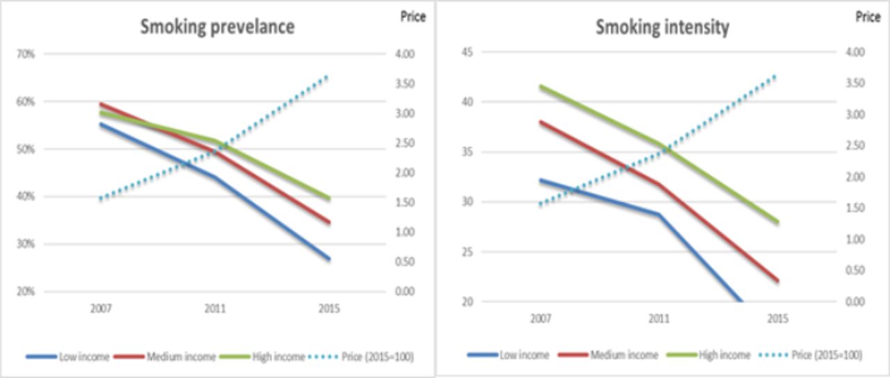
Smoking prevalence decreases in all income groups as cigarette prices increase, and the decrease in prevalence is higher among households in the high-income group (figure 1). Additionally, the difference in smoking prevalence by income group increases over time as cigarette prices increase.

Smoking prevalence and smoking intensity trends by income group.
It is the same case for smoking intensity trends by income group. High-income households smoked a greater quantity of cigarettes, compared with middle-income and low-income households. The quantity of cigarettes consumed decreased, but the differences in the quantities of consumption between different income groups increased over time as cigarette prices increased. Reductions in prevalence and intensity were more pronounced in the low-income group, especially in the years after introducing specific excise on cigarettes in 2009.
Notes: smoking prevalence is defined as the share of the households with positive tobacco consumption, while smoking intensity represents the number of cigarettes packs per household with positive expenditures on cigarettes per month. Cigarette prices are defined as municipality/year average cigarettes’ unit values (ratio between total expenditure and quantity) and expressed in real terms (2015=100).
Smoking households spend 4.7% of their budget on cigarettes (table 2). Subset of smoking households has a 17.7% higher total household expenditure (1812.5 vs 1544.7 BAM) and higher total expenditure per capita than all households (562.9 vs 591.5 BAM). Therefore, differences are more pronounced for total household expenditure because of the higher average number of household members among smoking households. The adults represent about 86% of the household members. Mean years of education is less than 8 years and suggest that on average household members have not even finished primary school. About 39.3% of all households are from urban areas, while the share of smoking households from urban areas is 1.7 percentage points higher. Approximately 59.3% of all households and 71.3% of smoking households have at least one person employed, while 22.5% of all households and 16.3% of smoking households have at least one person self-employed.
Descriptive statistics of household variables (monthly data)
Prevalence (probability) elasticity
The results of the estimation of prevalence elasticity (logit model) by income group and for all households are presented in table 3.18 19
Estimation of the prevalence elasticity
Probability that one of household members smokes is higher if the number of household members is higher and has a higher share of males and adults. Education level has a statistically significant impact on the smoking prevalence. The results suggest that more educated households are less likely to smoke compared with households whose members have incomplete or primary school. Also, households with finished primary school are more likely to smoke compared with those that did not finish that level of education. For almost all income groups, the households whose members, on average, have completed secondary (4 years) or higher education level are less likely to smoke compared with household whose members have unfinished primary school. Households from the urban areas have the higher propensity to smoke, with the exception of low-income households. Households in FB&H South region have higher propensity to smoking if we analyse all households, but for high-income group, only households in the RS East region have the lower propensity to smoking compared with households from other regions. The ‘unemployed’ households have more propensity to smoke compared with ‘pensioner’ and ‘self-employed’ households. The ‘employed’ households from high-income group are more likely to smoke.
Price and income elasticities are statistically significant and have expected signs for all income groups and on aggregate level. The results of the estimation of elasticities for all households suggest that increase in cigarette prices by 1% led to decrease in propensity to smoking by 0.554%, while increase in household income by 1% increases the propensity to smoking by 0.383%. Prevalence elasticities by income group show that the households that belong to the low-income group are the most responsive to price changes. Ten per cent price increase would result in a reduction in smoking prevalence by 8.0% in the low-income group, in comparison with 5.4% and 3.3%, in the middle-income and high-income group, respectively. Also, income elasticity is higher for low-income groups, which means that increase in income increases smoking participation if households belong to the low-income group. Ten per cent income increase would result in an increase in smoking prevalence by 4.4% in the low-income group, in comparison with 4.1% and 3.6%, in the middle-income and high-income group, respectively.
Conditional (intensity) elasticity
The condition for applying the Deaton model is that the price variation between clusters is large enough, which implies that the share total price variation explained by variation between clusters should be more than 50%. Therefore, we regress the unit value of cigarettes, expressed in logarithm, on the cluster level dummies. The results indicate significant F-statistic (F (389, 9518)=85.81, Prob>F=0.000) and R-square of 0.78, which means that the unit values can be used for the purpose of examining price variation and to estimate price elasticity.
The regression results of the unit values equation (table 4) show that the coefficients for total expenditure (expenditure elasticity of quality) are significant at 1% and positive for all income groups. These results confirm quality shading and the adequacy of using the Deaton model, as it enables control for the quality effect. Unit value is lower in larger households. Compared with the household level and high-income group, the increased number of household members in the low-income group has a lower impact on decreasing the price paid for cigarette pack. The reason is the fact that low-income households smoke less expensive cigarettes (table 1), so there is less space to find less expensive cigarettes. Male ratio is significant only at all household levels and suggests that households with higher share of men buy less expensive cigarettes. Except for low-income households, adult ratio has a statistically significant and negative impact on unit value paid for cigarettes. It shows that households with higher share of adults buy less expensive cigarettes. At the all-household level, the coefficient of mean education indicates that households whose average education is higher spend more money on a cigarette pack. The significance and sign of the maximum education variable imply that households with more educated members buy more expensive cigarettes, with the exception of the low-income group, as well as the households from urban areas. The ‘pensioners’ type of households spends less money on the cigarette packs compared with the ‘employed’ ones, with the exception of those from low-income group. The same goes for ‘self-employed’ households belonging to the middle-income group. The difference between the ‘unemployed’ and ‘employed’ households is not statistically significant, although the sign is, as expected, negative, except for high-income groups. The reasons may be the high level of informal unemployment,20 and very high personal transfers from abroad,21 characteristic of the Western Balkan countries, which sometimes obscures the true picture of socioeconomic status.
Unit value and budget share equations from Deaton model
As estimated coefficients from the budget share equation show (table 4), households with higher levels of expenditure as well as larger households that belong to the low-income group spend a smaller budget share on cigarettes. The opposite holds for households with higher share of men and higher share of adults, except for the middle-income group. More educated low-income households and households belonging to the middle-income group with the most educated members who have the higher level of education spend a smaller budget share on cigarettes. The ‘unemployed’ households spend greater budget share, while ‘self-employed’ spend smaller budget share on cigarettes compared with the ‘employed’ households. Cluster fixed effects are significant for both, unit value and budget share equation and indicate substantial variability in the unit value and budget shares between the clusters.
SEs for both price and expenditure elasticity are calculated using bootstrap procedure. The results are presented in table 5 and show that an increase in cigarette prices has the strongest effect on the quantity consumed by smokers who smoke in the low-income group – an increase in cigarette prices of 10% would decrease their cigarette quantity demanded by 6.1%. The corresponding change in the high-income group would be 3.6%. Also, conditional income elasticity of demand for cigarettes is lower if the household belongs to the high-income group.
Prevalence, conditional and total elasticities by income group
Total elasticity
The total price elasticity of smoking is very high (table 5). An increase in cigarette prices by 10% leads to a decrease in cigarette consumption by 10.1%. Roughly, about 55% of the negative effect of price growth on the overall demand comes from a decrease in smoking prevalence and 45% from the decrease in the quantity of cigarettes consumed by those who smoke. However, an increase in income by 10% leads to an increase in cigarette consumption by about 8.1%.
Estimated price elasticities show that low-income groups respond relatively more than others to changes in prices, both in terms of smoking participation and smoking intensity as well as to changes in income. Ten per cent price increase would reduce consumption of low-income households by 14%, as opposed to 9.9% and 7% for middle-income and high-income households, respectively. Similarly, 10% increase in income would increase consumption of the low-income group by 9.1%, in comparison with 7.9% and 7.4% for middle-income and high-income households, respectively.
We used bootstrapped SEs using 1000 repetitions to test for significant differences between price and income elasticities by different income groups. Regarding prevalence elasticity, the results showed that significant differences in estimated price elasticity exists, but the difference in estimated income elasticities by income group is not statistically significant. The results for conditional elasticity showed that the only statistically significant difference in estimated elasticity exists between price elasticity for low-income and middle-income group and between low-income and high-income groups. The statistically significant difference in total price elasticity exists between all income groups, while the difference in total income elasticity is significant between low-income and high-income groups.
Therefore, it can be concluded that low-income households are more responsive to the increase in cigarette prices by decreasing the demand for cigarettes compared with the middle-income and high-income group. Also, if income increases, low-income households increase the demand for cigarettes to a greater extent compared with high-income households.
Simulation of the impact of tax increase on consumption and government revenue
Based on the available administrative data and the estimated elasticities, table 6 outlines the impact of an increase in the specific excise tax and cigarette prices on cigarette consumption and government revenue from cigarettes assuming the scenarios of an increase in specific excise by 25% in 2019 compared with 2018.22
Projected impact of 25% specific excise tax increase on consumption and government revenue by income group
The simulation shows that an increase in specific excise by 25% in 2019 compared with 2018 would decrease cigarette consumption by 14.8%, while public revenue would increase by 2.3%. The low-income group would experience the greatest reduction in consumption (21.8%), which would also reduce their tax burden by 6.2%. However, while the middle-income and high-income group would also reduce consumption, the tax collection from these two groups would increase and more than compensate for the reduction in revenues from the low-income group, which would lead to an overall revenue gain of 2.3%.
Discussion and conclusions
This paper provides a unique HBS data-based estimation of price and income elasticity of the demand for cigarettes by different socioeconomic groups in B&H as well as elasticity estimation divided into prevalence and intensity elasticity. The estimated price elasticity is −1.01 and implies that an increase in cigarette prices by 10% leads to a decrease in cigarette consumption by 10.1%. Compared with the price elasticity estimates for Serbia,23 Montenegro24 and Croatia,25 where unconditional (total) price elasticity amounted to −0.64 to –0.8 and −1.38, respectively, it can be concluded that our estimated price coefficient is in line with research in similar neighbouring countries. Roughly about 55% of the negative effect of price growth on the overall demand comes from a decrease in smoking prevalence and 45% from a decrease in the quantity of cigarettes consumed by those who smoke. An increase in income by 10% leads to an increase in cigarette consumption by about 8.1%. Based on analysis of HBS data from 2007, 2011 and 2015 average number of cigarette packs consumed (per household) is decreasing in all income groups, but the decrease is much more evident in the low-income group.
Changes in prices and income have different impacts on tobacco consumption and prevalence by different socioeconomic groups. Low-income households are most responsive to changes in prices and would benefit most from higher cigarette prices in the long term: smoking prevalence would decrease by 8% in case of 10% price increase. It is obviously different compared with the middle-income and high-income group that would in the same scenarios have a decrease in prevalence of 5.4% and 3.3%, respectively. Also, the cigarette quantity demanded by low-income households responds more and significantly differently due to the increase in cigarette prices by 10%. It decreases by 6% compared with 4.5% and 3.7% as it is the case for the middle-income and high-income group. These results are in line with similar research from LMIC presented in introduction.7–9 Differences in income elasticity by income group are not statistically significant.
Tax simulation model revealed that more aggressive excise tax increase in government revenues from tobacco would see a slight increase of 2.3%. Low-income households would benefit most from higher cigarette taxes and prices, since the increase in excise taxes would reduce cigarette consumption most in this socioeconomic group compared with the middle-income and high-income group. This suggests that significant tax and price increases can have a positive health impact, while contributing to public revenues and increasing the progressivity of the tobacco tax system in B&H.
Limitations
B&H does not have a household survey on an annual basis. So far, household surveys have been carried out four times, in 2004, 2007, 2011 and 2015. The first survey could not be considered due to the low quality and reliability. However, the results of our survey are confirmed by earlier research in the LMICs. Justification for implementing policy of increasing the prices tobacco and tobacco products is also confirmed by the obvious benefits of decreasing the cigarette demand in B&H.
What this paper adds
Our study provides important empirical estimations of prevalence and intensity (conditional) elasticity of demand for cigarettes by income group in relation to the change in prices. We found out that an increase in cigarette prices by 10% leads to a decrease in cigarette consumption by 10.1%. Roughly, about 55% of the negative effect of price growth on the overall demand comes from a decrease in smoking prevalence and 45% from the decrease in the quantity of cigarettes consumed by those who smoke. An increase in income by 10% leads to an increase in cigarette consumption by about 8.1%. Low-income households are most responsive to changes in prices and income and would benefit most from higher cigarette prices in the long term. The tax simulation shows that an increase in specific excise by 25% in 2019 compared with 2018 would decrease cigarette consumption by 14.8% while public revenue would increase by 2.3%. The low-income group would experience the greatest reduction in consumption.
To the best of our knowledge, no existing studies in Bosnia and Herzegovina (B&H) have estimated the prevalence and intensity elasticity of demand for cigarettes in relation to the change in prices and income. Also, this is the first price and elasticity estimation of demand for cigarettes by income group. It demonstrates that the demand for cigarettes is responsive to its prices and income increase and that an increase in cigarette prices would reduce demand for cigarettes in B&H, while the low-income group would benefit most.
Data availability statement
Data are available on reasonable request. Data are available on reasonable request from the Agency of Statistics of Bosnia and Herzegovina.
Ethics statements
Patient consent for publication
Ethics approval
This study does not involve human participants.
Footnotes
Contributors All authors contributed to this manuscript. Author acting as guarantor is DG.
Funding This research is funded by the University of Illinois at Chicago’s Institute for Health Research and Policy through its partnership with Bloomberg Philanthropies.
Competing interests None declared.
Provenance and peer review Not commissioned; externally peer reviewed.